
Project Overview
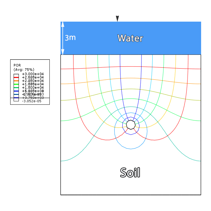
In this tutorial, the flow of groundwater through soil is simulated using Abaqus. The main objective is to analyze the seepage behavior and obtain the flow lines and equipotential lines in the soil domain.
This example is based on Example 9.11 from the Sam Helwany book. A horizontal drainage pipe is located below the ground surface, and the groundwater flows through the soil toward the drainage pipe.
Model Description
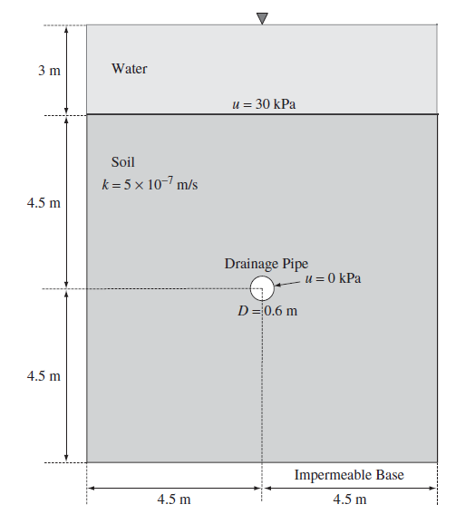
A long horizontal drainage pipe is located at a depth of 4.5 m below the ground surface. The drainage pipe has a diameter of 0.6 m.
Groundwater Flow
The seepage problem represents the flow of water through the soil toward the drainage pipe. The water pressure at the top surface of the flow domain is defined using a pore water pressure boundary condition.
The 3-m-deep water on top of the soil is replaced by a pore water pressure boundary condition of u = 30 kPa at the top surface of the flow domain.
Drainage Pipe
The drainage pipe acts as the outlet for the groundwater. The pore water pressure along the perimeter of the drain is set equal to zero.
This condition allows the groundwater to flow toward the drainage pipe and represents the hydraulic condition at the drain.
Soil Permeability
The permeability coefficient of the soil is defined as 5 × 10⁻⁷ m/s. This parameter controls the rate at which water flows through the soil during the seepage analysis.
The weight of the water is applied using gravity loading, allowing the effect of the water weight to be included in the groundwater-flow analysis.
Boundary Conditions
Appropriate hydraulic boundary conditions are applied to reproduce the groundwater-flow problem.
The two vertical sides and the bottom side of the flow domain are defined as impermeable boundaries. Therefore, water can flow through the soil toward the drainage pipe but cannot pass through these boundaries.
Seepage Analysis
The seepage analysis is performed in Abaqus to determine the groundwater-flow behavior within the soil domain. The numerical results are then used to visualize the direction of water flow and the distribution of hydraulic potential.
Flow Lines
The flow lines represent the paths followed by groundwater as it moves through the soil toward the drainage pipe. They provide a graphical representation of the direction of groundwater flow.

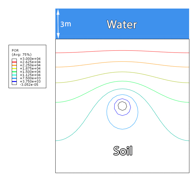
Equipotential Lines
The equipotential lines connect points having the same hydraulic potential. These lines illustrate the distribution of hydraulic head within the soil surrounding the drainage pipe.
Flow Net
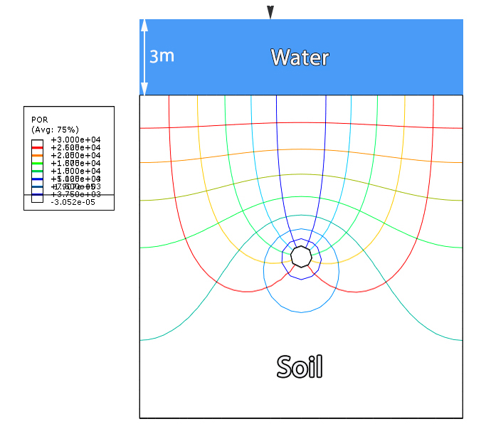
The flow lines and equipotential lines are used together to construct the flow net. The flow net provides a graphical representation of the groundwater seepage pattern through the soil toward the drainage pipe.
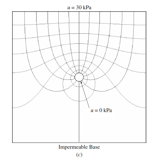
Results
The Abaqus results are used to visualize the groundwater-flow pattern and to obtain the flow lines and equipotential lines.
The resulting flow net provides a clear representation of how groundwater moves through the soil toward the horizontal drainage pipe.
What You Will Learn
- How to model groundwater seepage through soil in Abaqus.
- How to model a horizontal drainage pipe.
- How to define pore water pressure boundary conditions.
- How to define zero pore water pressure at a drainage boundary.
- How to define soil permeability in Abaqus.
- How to apply gravity loading to account for the weight of water.
- How to define impermeable boundaries for a seepage problem.
- How to obtain groundwater flow lines.
- How to obtain equipotential lines.
- How to construct a flow net for groundwater flow.
Key Features
- Groundwater seepage analysis.
- Example 9.11 from the Sam Helwany book.
- Horizontal drainage pipe.
- Drainage pipe diameter of 0.6 m.
- Drainage pipe located 4.5 m below the ground surface.
- 3-m-deep water represented by a pore water pressure boundary condition.
- Top pore water pressure of 30 kPa.
- Zero pore water pressure along the drain perimeter.
- Soil permeability of 5 × 10⁻⁷ m/s.
- Gravity loading for the weight of water.
- Impermeable vertical and bottom boundaries.
- Flow-line visualization.
- Equipotential-line visualization.
- Flow-net construction.
- Abaqus CAE model.
- Abaqus INP file.
- Step-by-step video tutorial.
Project Information
Important information about this project
Payment & Support
Need help with this tutorial?
Free Tutorial
This Abaqus tutorial is available free of charge.
Need Help?
If you have any questions about this tutorial, please contact us by email.
saeedofmoeini@gmail.com
There are no reviews yet.