
Project Overview
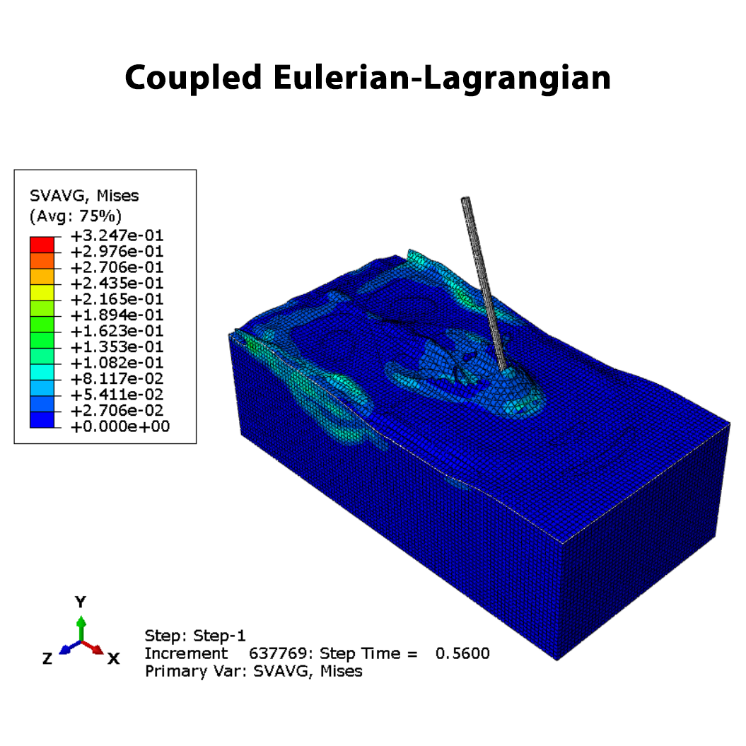
In this tutorial, the entry of a pendulum into water is simulated using the Coupled Eulerian-Lagrangian (CEL) method in Abaqus. The simulation focuses on the interaction between the pendulum and water during its oscillating motion.
In this example, the reciprocating motion of a pendulum is simulated as it enters the water and causes the water to become turbulent. The motion of the pendulum and its interaction with the water are investigated during the simulation.
Problem Description
In this problem, a pendulum is initially positioned at an angle of 60 degrees with respect to the vertical axis. The pendulum then moves under the action of its own weight, causing it to undergo an oscillating motion.
During its reciprocating motion, the pendulum enters the water, resulting in significant interaction between the pendulum and the water and causing the water to become turbulent.
As time passes, the amplitude of the pendulum's oscillation gradually decreases until the pendulum eventually comes to a complete stop.
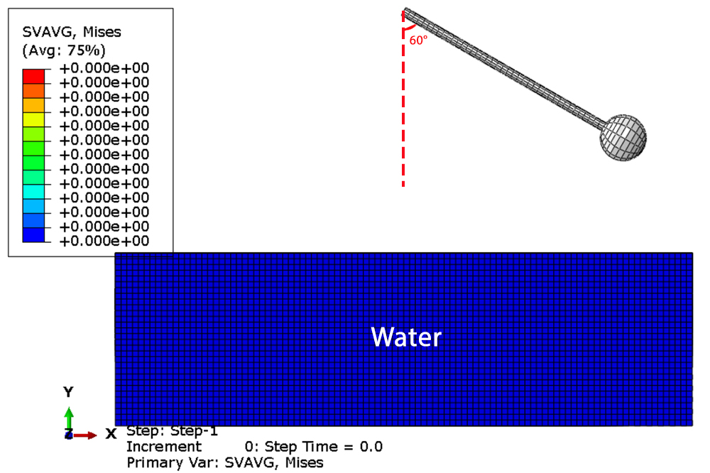
Coupled Eulerian-Lagrangian Method
To simulate the interaction between the pendulum and the water, the Coupled Eulerian-Lagrangian (CEL) method is used in Abaqus. This method is suitable for problems involving large deformation and complex fluid-structure interaction.
In this simulation, the motion of the pendulum is modeled together with the behavior of the water so that the interaction between the two can be captured during the pendulum's oscillating motion.
Water Properties
The water is defined using the required physical properties for the Eulerian fluid simulation.
- Density: 1000 kg/m³
- Viscosity: 0.001 Pa·s
- Speed of sound: 1500 m/s
Simulation Results
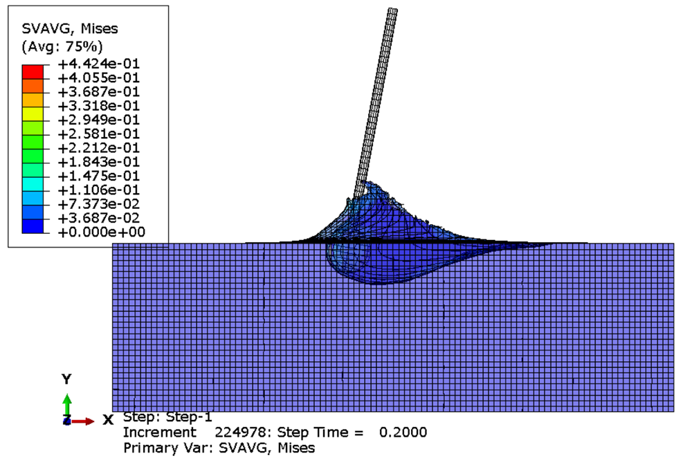
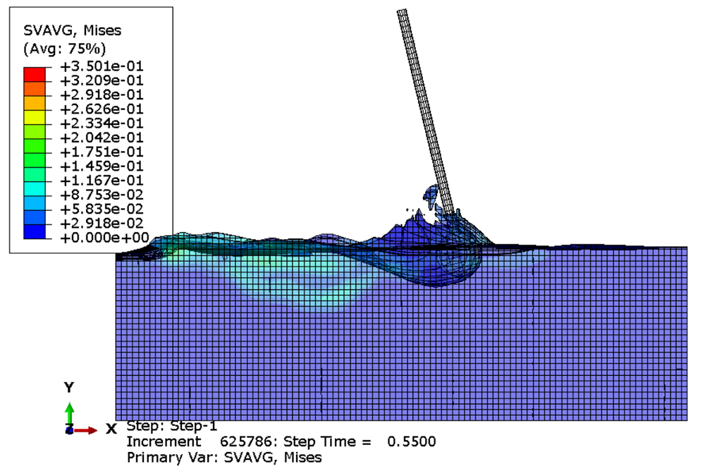
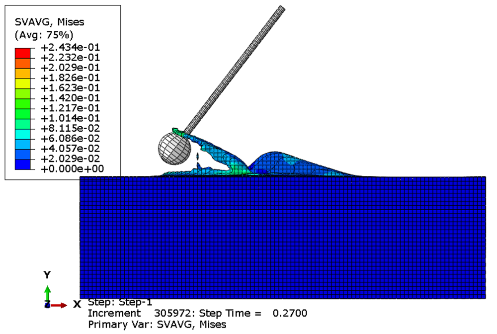
The simulation results show the motion of the pendulum as it enters and exits the water during its oscillation. The behavior of the water and the development of turbulence can also be observed throughout the simulation.
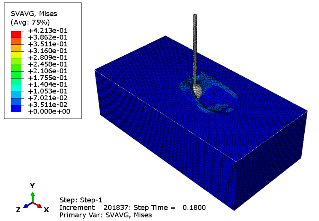
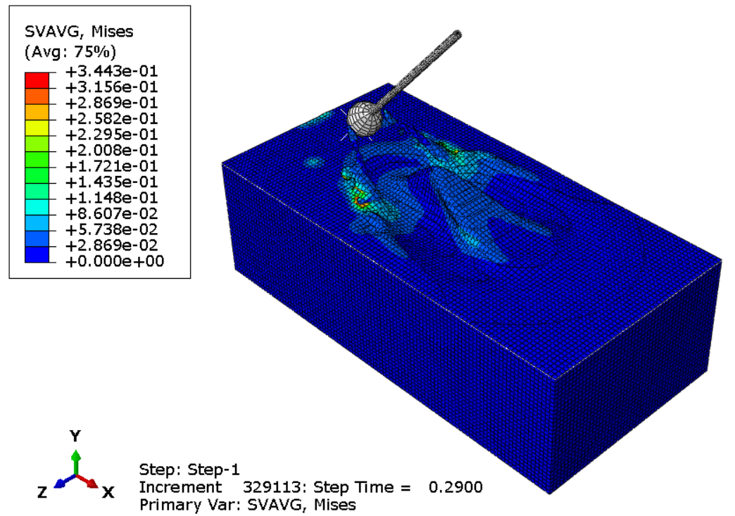
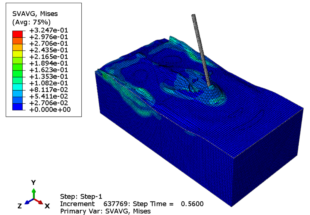
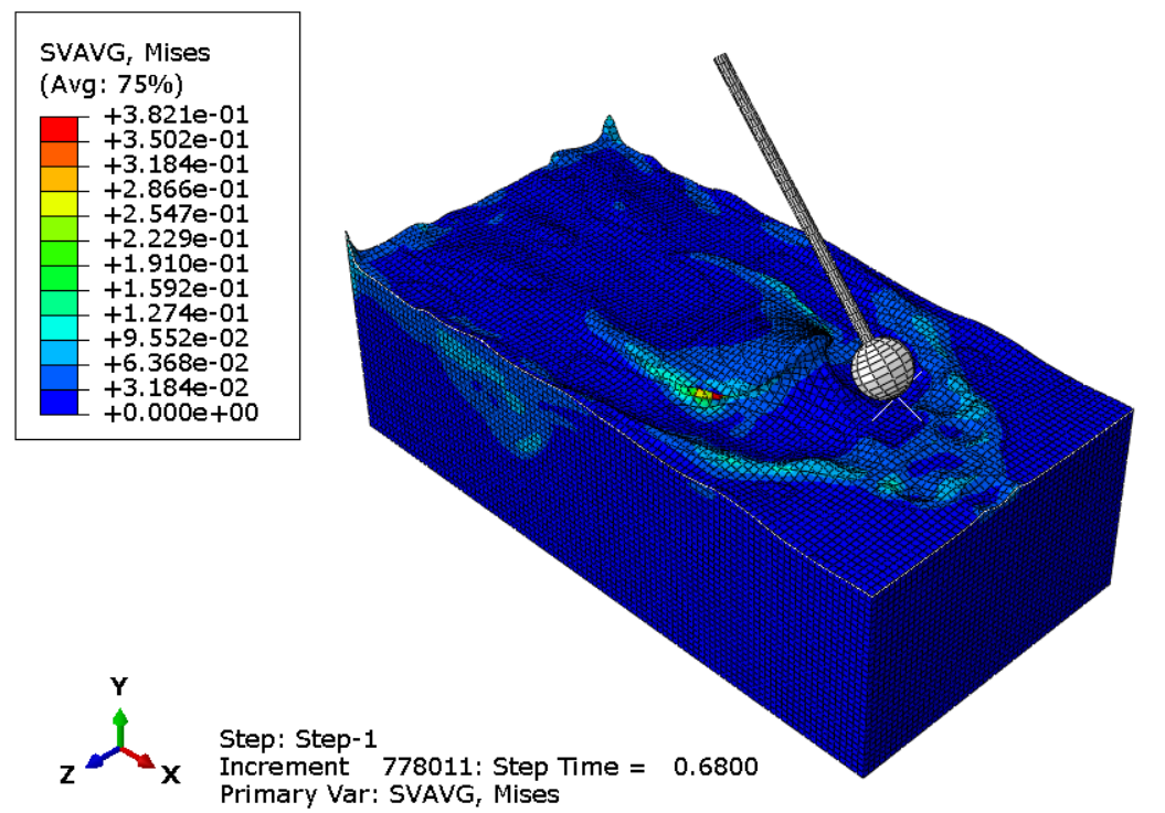
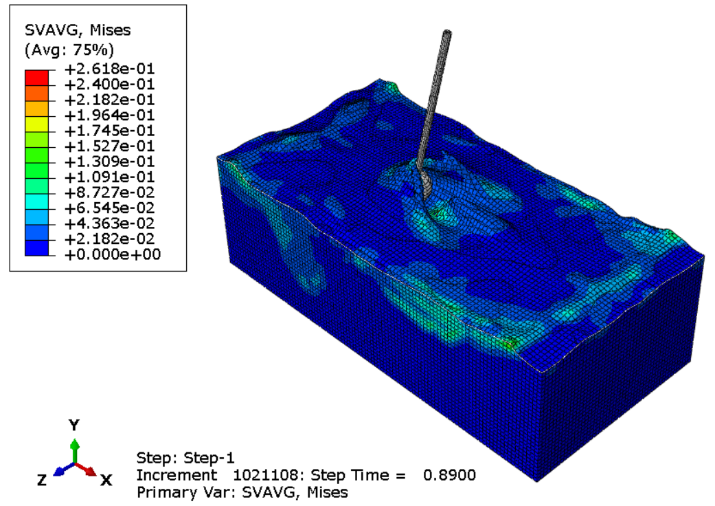
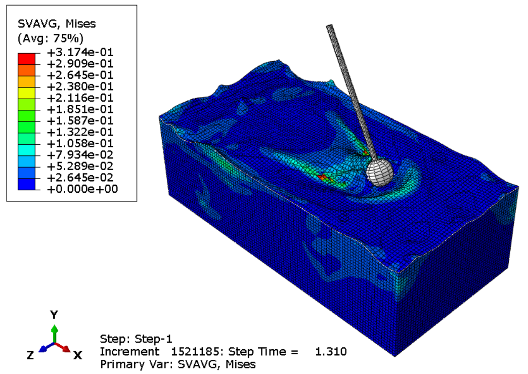
Different stages of the simulation are presented at various times, including 0.18 s, 0.29 s, 0.56 s, 0.68 s, 0.89 s, and 1.31 s, allowing the evolution of the pendulum motion and water behavior to be observed.
What You Will Learn
- How to model a pendulum entering water in Abaqus.
- How to use the Coupled Eulerian-Lagrangian (CEL) method.
- How to simulate fluid-structure interaction.
- How to model the oscillating motion of a pendulum.
- How to simulate the interaction between the pendulum and water.
- How to observe the turbulent behavior of water.
- How to analyze the motion of the pendulum during water entry.
Key Features
- Coupled Eulerian-Lagrangian (CEL) analysis.
- Pendulum entry into water.
- Fluid-structure interaction.
- Initial pendulum angle of 60 degrees.
- Oscillating motion under the action of gravity.
- Water turbulence caused by pendulum motion.
- Simulation of the gradual reduction in oscillation amplitude.
- Observation of the pendulum until it comes to a complete stop.
- Free Abaqus tutorial.
Project Information
Important information about this project
Payment & Support
Need help with this tutorial?
Free Tutorial
This Abaqus tutorial is available free of charge.
Need Help?
If you have any questions about this tutorial, please contact us by email.
saeedofmoeini@gmail.com
There are no reviews yet.