Period of the pendulum using the Abaqus software and Analytical Solution

Project Overview

In this Abaqus tutorial, the period of a pendulum is calculated using both the analytical solution and the Abaqus software.

The main objective of this tutorial is to first calculate the period of the pendulum using the analytical solution, then obtain the period using Abaqus, and finally compare the results obtained from both approaches.

Pendulum Model

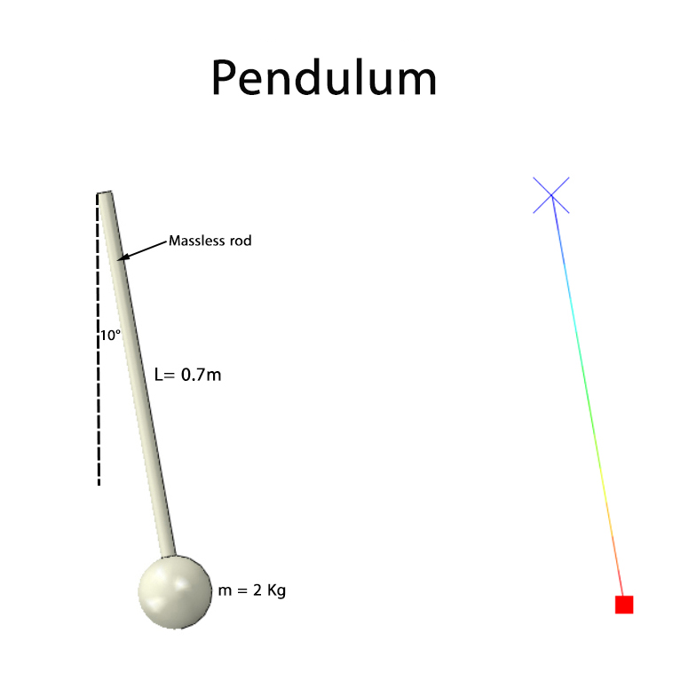
In this problem, the initial angle of the pendulum is 10 degrees, the length of the pendulum is 0.7 m, and the mass of the ball is 2 kg.

These parameters are used to calculate the period of the pendulum using the analytical solution and the Abaqus software.

Calculation of the Period

The period of a pendulum is the amount of time required to complete one full swing, or in other words, the time required for the pendulum to return to its original position.

First, the period of the pendulum is calculated using the analytical solution. Following that, the same problem is modeled in Abaqus and the period is obtained from the numerical simulation.

Analytical Solution

The period of the pendulum is first calculated using the analytical solution.

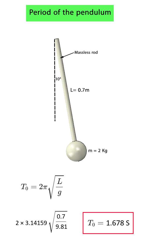
For a simple pendulum, the period is determined based on the length of the pendulum and the gravitational acceleration. Since the initial angle of the pendulum is 10 degrees, the small-angle approximation can be used to calculate the period.

Using the pendulum length of 0.7 m and the standard gravitational acceleration, the analytical solution gives a period of approximately 1.678 seconds.

This analytical value is used as the reference result for comparison with the period obtained from the Abaqus dynamic simulation.

Obtaining the Period in Abaqus

To obtain the period of the pendulum, a Dynamic, Explicit analysis is performed in Abaqus. The weight of the pendulum rod and a 2 kg mass are considered in the model, allowing the pendulum to undergo free vibration.

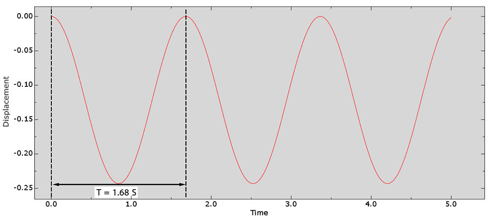
During the dynamic analysis, the motion of the 2 kg mass is recorded. The displacement-time response of the mass is then plotted to visualize the oscillatory motion of the pendulum.

Finally, the period of the system is determined from the displacement-time response by measuring the time interval between corresponding points of consecutive oscillations.

Comparison of Analytical and Abaqus Results

The period of the pendulum obtained from the analytical solution is 1.678 seconds.

The period obtained from the Abaqus software is 1.68 seconds.

As observed from the results, the period obtained from Abaqus is in very good agreement with that obtained from the analytical solution.

What You Will Learn

• How to model a pendulum in Abaqus.
• How to define the geometry and mass of the pendulum.
• How to define the initial angle of the pendulum.
• How to calculate the period using the analytical solution.
• How to obtain the period from an Abaqus simulation.
• How to compare Abaqus results with an analytical solution.
• How to evaluate the accuracy of a simple dynamic model using an analytical solution.

Key Features

• Pendulum dynamic analysis.
• Period calculation.
• Analytical solution.
• Abaqus numerical simulation.
• Comparison between analytical and Abaqus results.
• Initial angle of 10 degrees.
• Pendulum length of 0.7 m.
• Ball mass of 2 kg.
• Free Abaqus tutorial.