First Torsional Natural Frequency of a Cantilever Beam in Abaqus

Project Overview

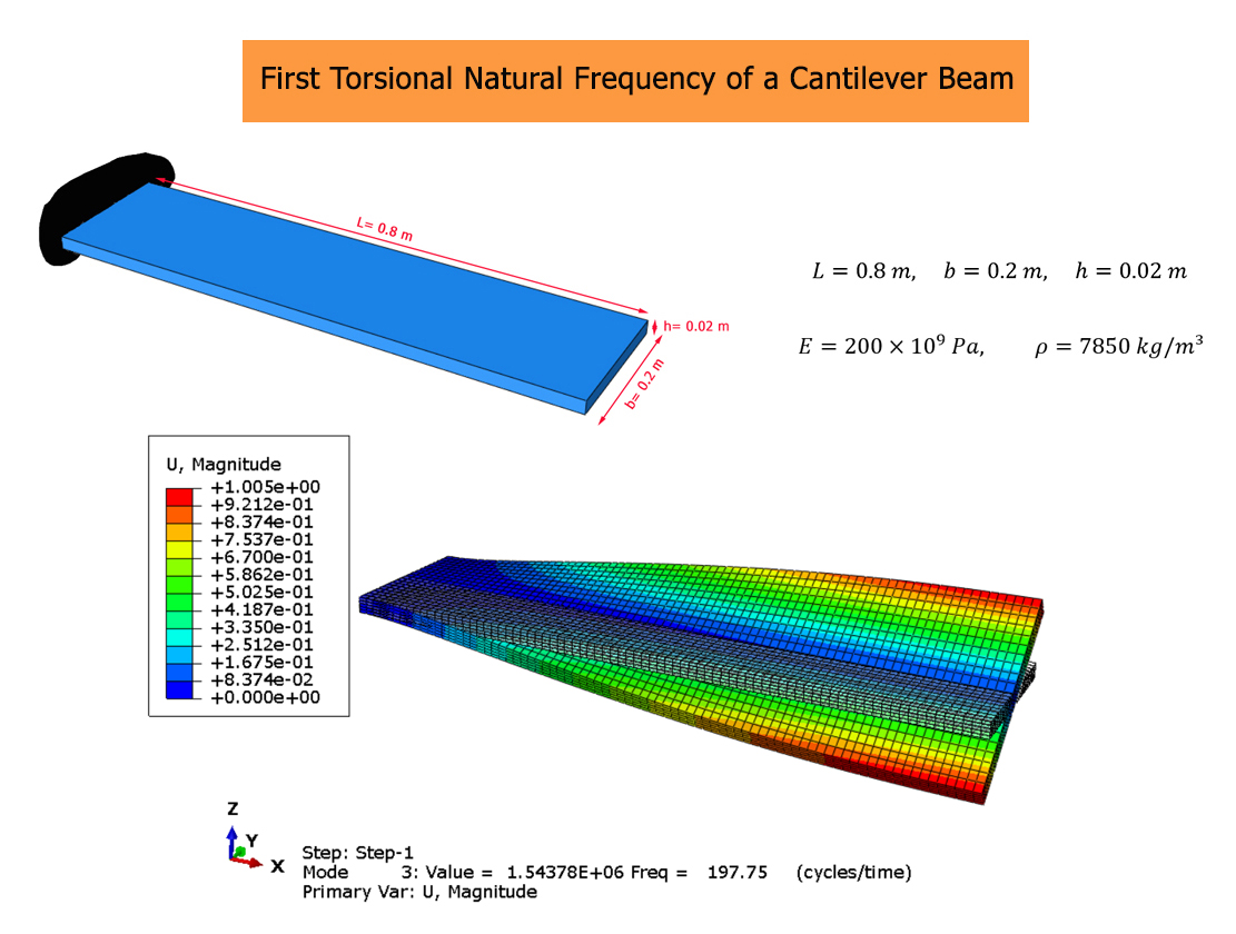
In this training, we calculate the first torsional natural frequency of a cantilever beam using the Abaqus software. The beam is modeled using two different finite element approaches: 3D solid elements and beam elements. The results obtained from both models are then compared with the Analytical Solution based on torsional vibration theory to evaluate the accuracy of the numerical results.

Model Description

The model consists of a steel cantilever beam with a length of 0.8 m, a width of 0.2 m, and a height of 0.02 m.

The material properties are defined as follows: Young's modulus is 200 GPa, Poisson's ratio is 0.3, and the material density is 7850 kg/m³.

One end of the beam is fixed, while the other end is free to vibrate. The objective is to determine the first torsional natural frequency and compare the results obtained using solid and beam elements with the analytical solution.

Abaqus Simulation

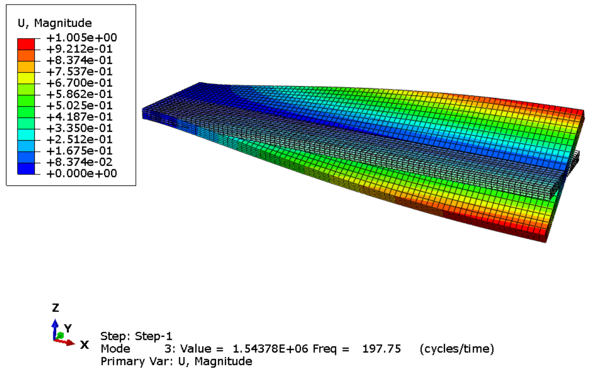
First, the cantilever beam is simulated using three-dimensional solid elements in Abaqus. A frequency analysis is performed to calculate the natural frequencies and corresponding mode shapes.

The torsional mode is identified by examining the deformation pattern of the beam. In this mode, the beam rotates around its longitudinal axis.

The first torsional natural frequency obtained from the solid element model is equal to 197.75 Hertz.

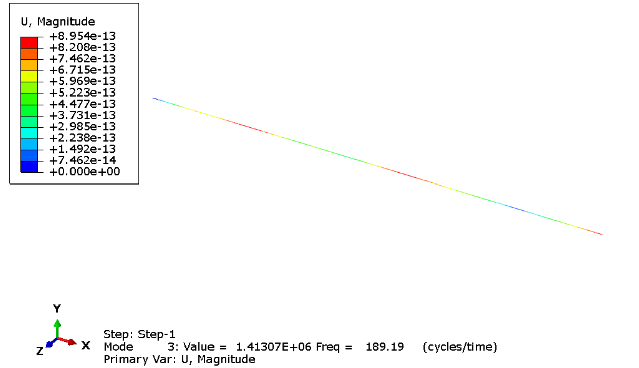
Next, the same cantilever beam is modeled using beam elements. The material properties, beam dimensions, and boundary conditions remain unchanged.

A frequency analysis is performed to obtain the first torsional natural frequency and its corresponding mode shape. The frequency obtained from the beam element model is 189.19 Hertz.

Analytical Solution

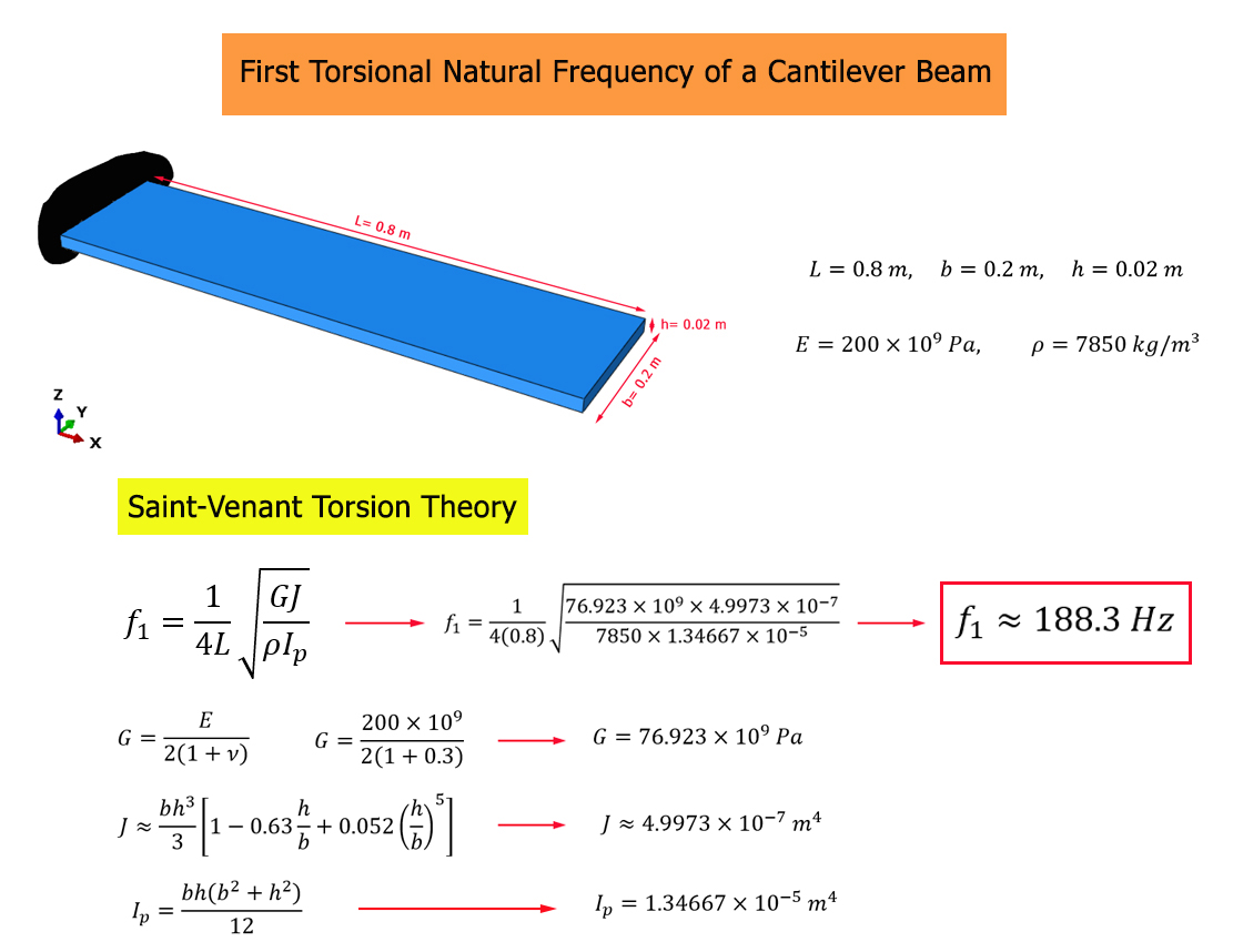
Next, the first torsional natural frequency of the cantilever beam is calculated using the Analytical Solution based on torsional vibration theory.

For a uniform shaft with one end fixed and the other end free, the first torsional natural frequency can be calculated using the following equation:

f₁ = (1 / 4L) √(GJ / ρI_p)

In this equation, G is the shear modulus, J is the Saint-Venant torsion constant of the cross-section, ρ is the material density, I_p is the polar second moment of area, and L is the beam length.

The shear modulus is calculated using Young's modulus and Poisson's ratio:

G = E / [2(1 + ν)]

For the rectangular cross-section considered in this problem, the torsion constant is calculated using an approximate analytical expression.

The first torsional natural frequency obtained from the Analytical Solution is approximately 188.3 Hertz.

Comparison of Results

The results obtained from the two Abaqus models are compared with the Analytical Solution based on torsional vibration theory.

The first torsional natural frequency obtained from the solid element model is 197.75 Hz, while the beam element model gives 189.19 Hz. The frequency obtained from the Analytical Solution is 188.3 Hz.

The difference between each Abaqus result and the Analytical Solution is presented in the following table.

What You Will Learn

• How to model a cantilever beam in Abaqus using solid elements.
• How to model a cantilever beam using beam elements.
• How to define material properties and density in Abaqus.
• How to apply boundary conditions to a cantilever beam.
• How to perform a natural frequency analysis.
• How to obtain natural frequencies and mode shapes using Abaqus.
• How to identify the first torsional mode from its mode shape.
• How to calculate the first torsional natural frequency using torsional vibration theory.
• How to compare solid and beam element results with the Analytical Solution.
• How to evaluate the accuracy of different finite element models.

Key Features

• Torsional vibration analysis of a cantilever beam.
• Three-dimensional solid finite element model.
• Beam element finite element model.
• Steel material properties.
• First torsional natural frequency calculation.
• Analytical Solution based on torsional vibration theory.
• Identification of the first torsional mode shape.
• Comparison between solid and beam element results.
• Validation of numerical results against the Analytical Solution.
• Free Abaqus tutorial.