Price Free!

Product Overview

In this example, we intend to calculate the fluid front position over time in the dam break problem using the Abaqus software.

The water column is initially confined within the Eulerian domain. When gravity is applied, the water column collapses and the water flows across the ground. The movement of the fluid front is then tracked throughout the simulation.

Dam break problem and fluid front simulation in Abaqus
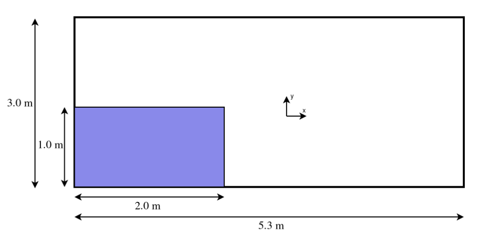
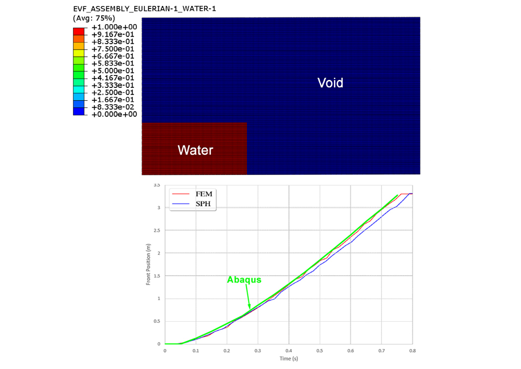
Dam break problem modeled using the Eulerian approach in Abaqus.

Eulerian Analysis

The dam break problem is modeled using an Eulerian domain, which provides the computational region in which the water can move during the simulation.

The Eulerian domain has a length and width of 5.3 m × 3 m. The initial water column has an elevation of 1 m.

Water Properties

The water is defined using the required physical properties for the Eulerian fluid simulation.

  • Density: 1000 kg/m³
  • Viscosity: 0.001 Pa·s
  • Speed of sound: 1500 m/s

Gravity Loading

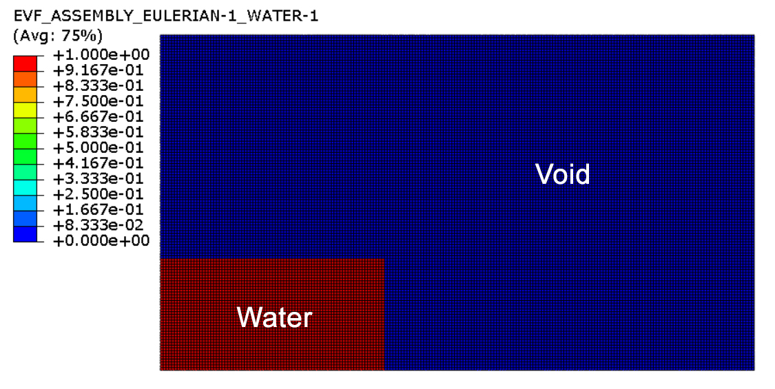
A gravity load is applied to the water column. Under gravity, the initially confined water collapses and flows along the ground inside the Eulerian domain.

Gravity loading applied to water column in dam break simulation
Gravity-driven collapse of the water column.

Fluid Evolution Over Time

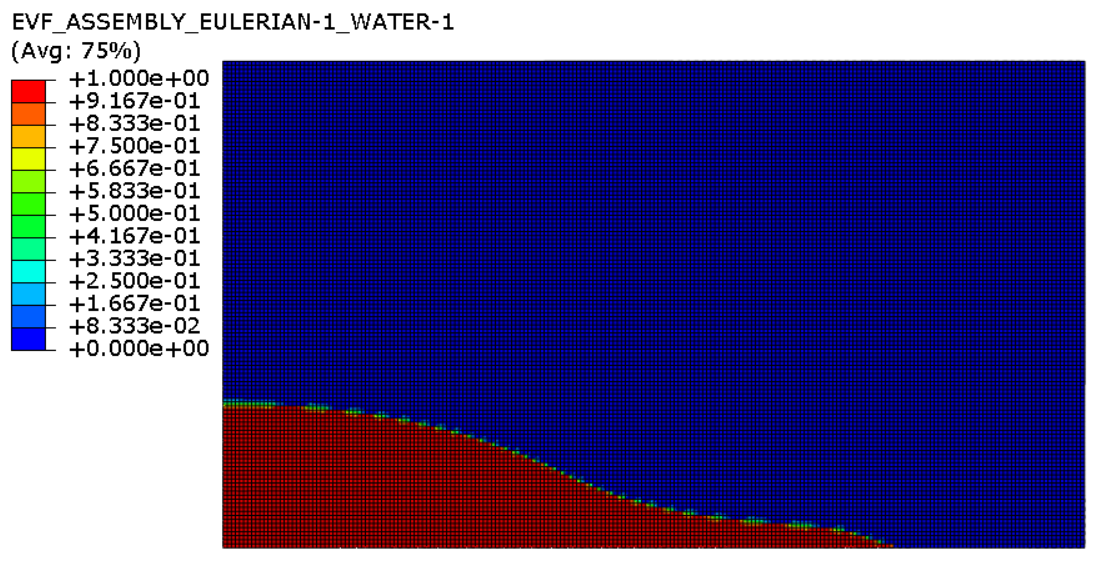
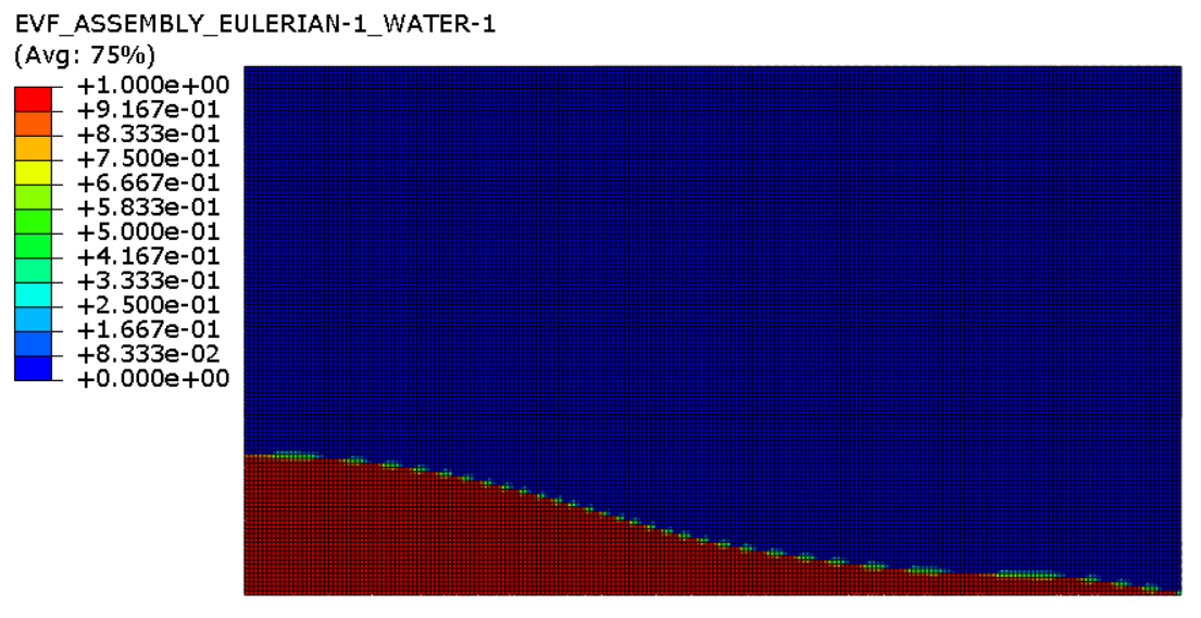
The deformation and movement of the water column are investigated at different time intervals. The evolution of the fluid front illustrates how the water propagates through the Eulerian domain after the collapse begins.

Dam break simulation at 0.25 seconds in Abaqus
Fluid configuration at T = 0.25 s.
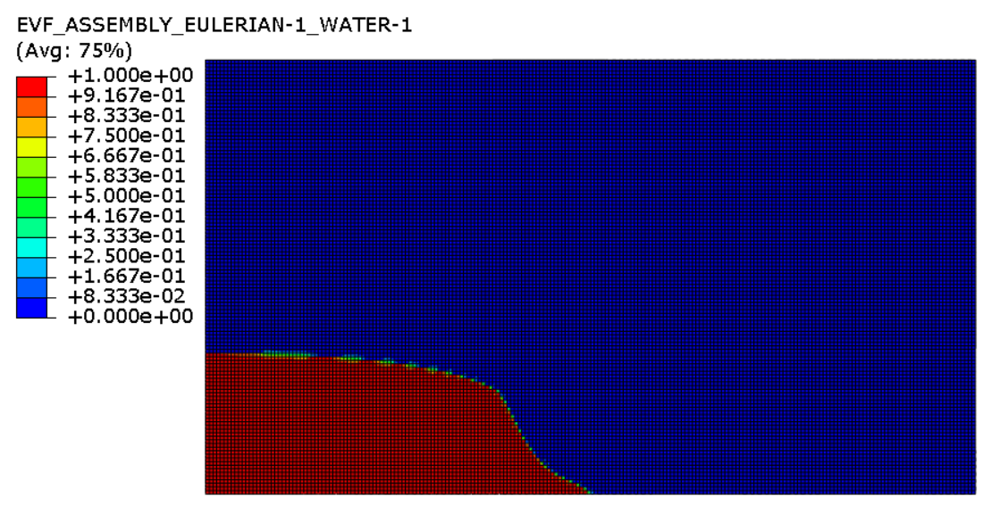
Dam break simulation at 0.4 seconds in Abaqus
Fluid configuration at T = 0.4 s.
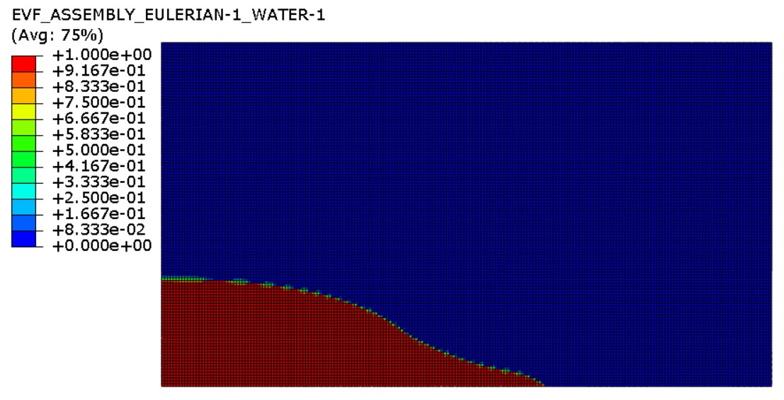
Dam break simulation at 0.55 seconds in Abaqus
Fluid configuration at T = 0.55 s.
Dam break simulation at 0.75 seconds in Abaqus
Fluid configuration at T = 0.75 s.

Fluid Front Position Over Time

The position of the fluid front is obtained at different time intervals during the dam break simulation.

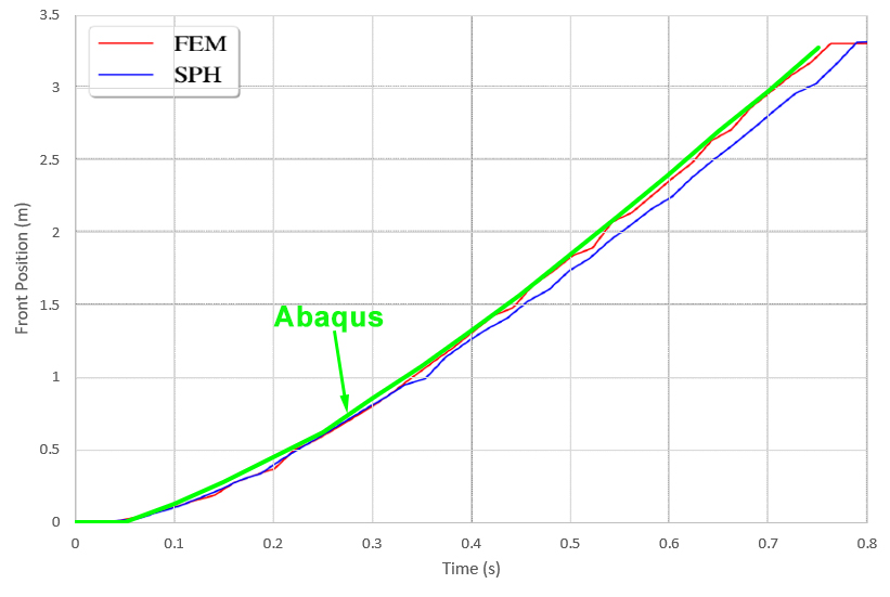
A fluid front position versus time diagram is plotted to describe the propagation of the water front after the initial collapse of the water column.

Fluid front position versus time diagram in dam break simulation
Fluid front position over time obtained from the Abaqus simulation.

Validation

This project has been validated by comparing the results obtained from the Abaqus software with the results reported in the reference article.

The comparison demonstrates that the numerical results are in good agreement with the reported results, confirming the ability of the model to reproduce the fluid-front propagation in the dam break problem.

Reference

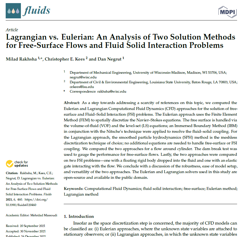
This project is based on a research article dealing with the dam break problem. The article is used as the reference for validating the numerical results obtained from Abaqus.

Research article used for validation of dam break simulation
Reference research article used for validation.

What You Will Learn

  • How to model a dam break problem in Abaqus.
  • How to perform an Eulerian fluid analysis.
  • How to define an Eulerian domain for fluid movement.
  • How to define water properties for the simulation.
  • How to apply gravity to an Eulerian water column.
  • How to investigate fluid propagation over time.
  • How to determine the fluid front position.
  • How to plot the fluid front position versus time.
  • How to compare numerical results with published results.
  • How to validate a dam break simulation using a research article.

Key Features

  • Dam break simulation in Abaqus.
  • Eulerian fluid analysis.
  • Gravity-driven water flow.
  • 5.3 m × 3 m Eulerian domain.
  • 1 m initial water column elevation.
  • Water density of 1000 kg/m³.
  • Water viscosity of 0.001 Pa·s.
  • Water speed of sound of 1500 m/s.
  • Fluid evolution at different time intervals.
  • Fluid front position calculation.
  • Fluid front position versus time diagram.
  • Comparison with published research results.
  • Validation of the Abaqus model.
  • Complete Abaqus model files.
  • Step-by-step video tutorial.
Files Included
What you will receive after purchase
File Type
Content
Description
🧩 Abaqus
CAE File
Complete Abaqus model
📄 Abaqus
INP File
Abaqus input file
📊 Excel
Numerical Results
Results extracted from the Abaqus analysis
📑 Document
Research Paper
Reference paper used for the project
🎥 Video
Full Video
Step-by-step explanation of the project

Project Information

Important information about this project

🎥
Video Tutorial Available
📦
Project Type Free Tutorial
💻
Abaqus Version Abaqus 2017
🌐
Language English
📥
Access Free

Payment & Support

Need help with this tutorial?

🎓

Free Tutorial

This Abaqus tutorial is available free of charge.

✉️

Need Help?

If you have any questions about this tutorial, please contact us by email.

saeedofmoeini@gmail.com

chat_bubble_outlineReviews

There are no reviews yet.

Be the first to review “Fluid front position over time in the dam break problem in Abaqus”

Your email address will not be published. Required fields are marked *