
Project Overview
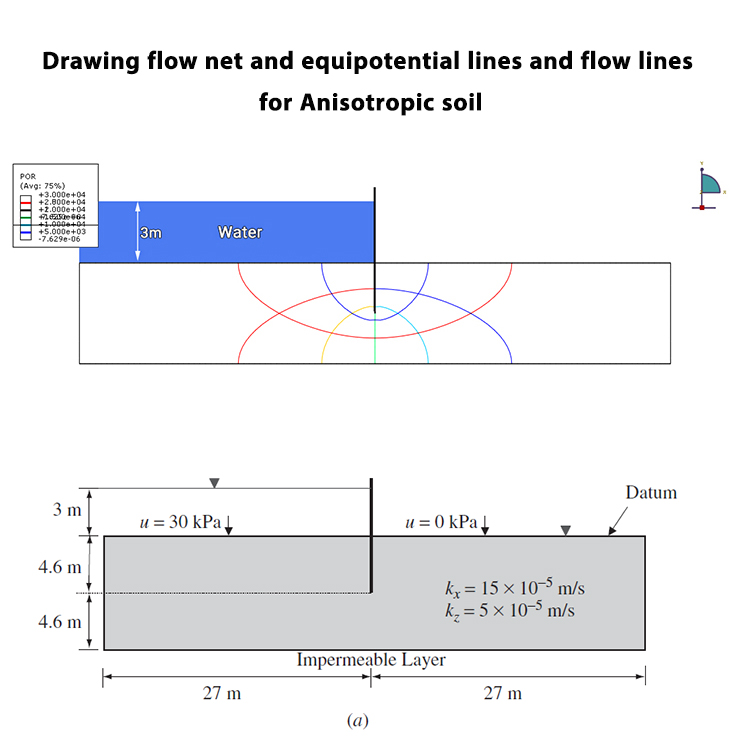
In this tutorial, the seepage behavior of anisotropic soil is simulated using Abaqus. The main objective is to obtain the flow lines and equipotential lines from the numerical analysis and use them to construct the flow net.
A flow net consists of two families of curves: flow lines and equipotential lines. These lines are used to visualize the direction of groundwater flow and the distribution of hydraulic head within the soil.
Model Description
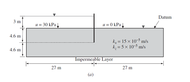
In this example, the soil is assumed to be anisotropic, meaning that its permeability is different in different directions. This condition affects the pattern of seepage and consequently the shape of the flow lines and equipotential lines.
Seepage Analysis
The seepage analysis is performed in Abaqus to determine the distribution of pore water pressure and hydraulic head within the soil domain.
The numerical model is defined using a coupled pore fluid and stress analysis, allowing the flow of water through the soil to be simulated directly in Abaqus.
Flow Lines
The flow lines represent the paths followed by water as it flows through the soil. These lines are obtained from the seepage analysis and are used to visualize the direction of groundwater flow.

Equipotential Lines
The equipotential lines connect points having the same hydraulic head. They provide information about the distribution of hydraulic potential throughout the soil domain.

Flow Net
The flow lines and equipotential lines are superimposed to form the flow net. The resulting flow net provides a graphical representation of the seepage pattern through the anisotropic soil.

Results
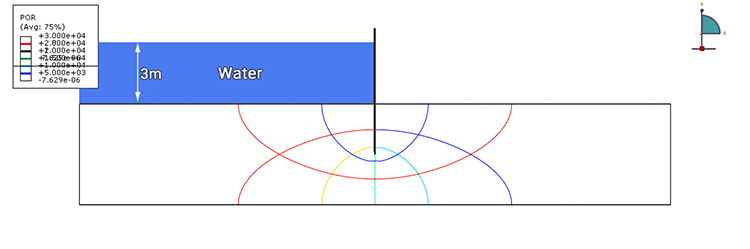
The Abaqus results are used to obtain the flow lines and equipotential lines and to construct the final flow net. This provides a clear visualization of the seepage behavior within the anisotropic soil.
The analysis demonstrates how Abaqus can be used to simulate groundwater flow through anisotropic soil and obtain the graphical information required for flow-net analysis.
What You Will Learn
- How to model anisotropic soil in Abaqus.
- How to perform seepage analysis in Abaqus.
- How to define permeability for anisotropic soil.
- How to obtain flow lines from Abaqus results.
- How to obtain equipotential lines from Abaqus results.
- How to superimpose flow lines and equipotential lines.
- How to construct a flow net for anisotropic soil.
- How to visualize groundwater flow through soil.
Key Features
- Anisotropic soil seepage analysis.
- Flow-line visualization.
- Equipotential-line visualization.
- Flow-net construction.
- Coupled pore fluid and stress analysis.
- Abaqus CAE model.
- Abaqus INP file.
- Step-by-step video tutorial.
- Free Abaqus tutorial.
Project Information
Important information about this project
Payment & Support
Need help with this tutorial?
Free Tutorial
This Abaqus tutorial is available free of charge.
Need Help?
If you have any questions about this tutorial, please contact us by email.
saeedofmoeini@gmail.com
There are no reviews yet.