
Project Overview
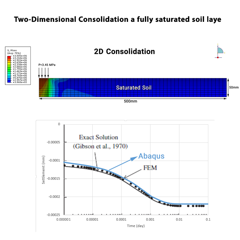
In this Abaqus tutorial, the two-dimensional consolidation of a fully saturated soil layer is simulated. The numerical results obtained from Abaqus are compared with the theoretical solution proposed by Gibson et al.
This example is based on Example 4.6 from Sam Helwany's book, in which the consolidation settlement at the center of a loaded strip is investigated as a function of time.
The purpose of this simulation is to verify the ability of Abaqus to reproduce the consolidation response of a saturated soil layer under a partially distributed surface load.

Two-dimensional consolidation model of a fully saturated soil layer.
Soil Layer and Loading
The soil layer has a finite thickness of 50 mm and extends infinitely in the horizontal direction.
A 50 mm-wide strip load is applied to the top surface of the soil layer. The magnitude of the applied load is 3.45 MPa.
Due to the symmetry of the problem, only one-half of the model needs to be considered in the finite element analysis.

Geometry, symmetry, and strip loading used in the consolidation model.
Soil Material Properties
The soil is assumed to behave as a linear elastic and fully saturated material.
- Young's modulus: 690 GPa
- Poisson's ratio: 0
- Permeability: 5.08 × 10⁻⁷ m/day
- Fluid specific weight: 272.9 kN/m3
These material parameters are selected according to the reference problem and are intended to reproduce the theoretical consolidation solution.
Finite Element Model
A two-dimensional plane strain finite element model with pore pressure degrees of freedom is used for the analysis.
The mesh is refined near the loaded region, where larger stress and deformation gradients are expected. Coarser elements are used farther away from the loading area.
The model represents a soil layer with infinite horizontal extension while using symmetry to reduce the computational domain.
Boundary Conditions
Appropriate mechanical and hydraulic boundary conditions are defined to reproduce the conditions of the reference consolidation problem.
- The bottom boundary is assumed to be smooth and impervious.
- The vertical displacement at the bottom boundary is constrained.
- The symmetry boundary is constrained against horizontal movement.
- The far-side boundary is constrained horizontally while remaining free to move vertically.
- Drainage is allowed through the appropriate drained boundary.
Consolidation Analysis
The problem is analyzed using six steps. In the first step, the applied load is gradually introduced with a magnitude of 3.45 MPa. During this step, no drainage is allowed through the top surface of the soil.
After the initial loading step, the actual consolidation process is simulated using five consecutive time steps. During these steps, excess pore pressure dissipates and the soil gradually undergoes consolidation settlement.
| Step | Purpose | Duration |
|---|---|---|
| Step 1 | Application of 3.45 MPa load with no drainage through the top surface | Initial loading step |
| Step 2 | Consolidation | 0.00001 day |
| Step 3 | Consolidation | 0.0001 day |
| Step 4 | Consolidation | 0.001 day |
| Step 5 | Consolidation | 0.01 day |
| Step 6 | Consolidation | 0.1 day |
The five consolidation steps are used to capture the dissipation of excess pore pressure and the corresponding settlement of the soil over time.

Six analysis steps used for loading and consolidation of the fully saturated soil layer.
Consolidation Settlement
The main output of the simulation is the consolidation settlement at the center of the loaded strip as a function of time.
The settlement obtained from Abaqus is compared with the Gibson theoretical solution.

Consolidation settlement at the center of the loaded strip as a function of time.
Comparison with Gibson's Solution
The numerical settlement history obtained from Abaqus is compared with the theoretical solution developed by Gibson et al.
This comparison provides a verification of the finite element model by evaluating how closely the Abaqus consolidation response follows the reference theoretical solution.

Six analysis steps used for loading and consolidation of the fully saturated soil layer.
What You Will Learn
- How to model a fully saturated soil layer in Abaqus.
- How to create a two-dimensional plane strain consolidation model.
- How to define a soil material with pore fluid.
- How to define soil permeability.
- How to define the fluid specific weight.
- How to use plane strain elements with pore pressure degrees of freedom.
- How to define mechanical boundary conditions.
- How to define hydraulic boundary conditions.
- How to apply a strip load to a saturated soil layer.
- How to simulate excess pore pressure dissipation.
- How to simulate consolidation settlement.
- How to obtain settlement as a function of time.
- How to compare Abaqus results with Gibson's theoretical solution.
Key Features
- Two-dimensional plane strain consolidation analysis.
- Fully saturated soil layer.
- Soil layer thickness of 50 mm.
- 50 mm-wide strip load.
- Applied load of 3.45 MPa.
- Linear elastic soil behavior.
- Young's modulus of 690 GPa.
- Poisson's ratio of 0.
- Permeability of 5.08 × 10⁻⁷ m/day.
- Fluid specific weight of 272.9 kN/m3.
- Plane strain elements with pore pressure degrees of freedom.
- Symmetry-based finite element model.
- Excess pore pressure dissipation.
- Consolidation settlement versus time.
- Comparison with Gibson's theoretical solution.
- CAE file.
- INP file.
- Excel file containing the results.
Project Information
Important information about this project
Payment & Support
Need help with this tutorial?
Free Tutorial
This Abaqus tutorial is available free of charge.
Need Help?
If you have any questions about this tutorial, please contact us by email.
saeedofmoeini@gmail.com
There are no reviews yet.